Tree, as a subtype of graph, is most commonly used data structure in computer science, with different variants for different purposes: search, range query, update, etc.
Heap, or priority queue, is a type of queue. I put it under tree category because in essense it maintains its property for being a “tree”.
It supports O(1) maximum/minimum value look up, O(logn) maximum value deletion/pop, O(logn) element insertion.
A type of priority queue.
Parent is bigger than its children.
class MinHeap:
	def heapify(self, array):
		"""Convert an random array into a heap."""
		for i in reversed(range(len(array) // 2)):
			self._siftdown(array, i)

	def pop(self, heap):
		"""Pop the smallest item off the heap, maintaining the heap invariant. """
		lastelt = heap.pop()  # raises appropriate IndexError if heap is empty
		if heap:
			returnitem = heap[0]
			heap[0] = lastelt
			self._siftdown(heap, 0)
			return returnitem
		return lastelt

	def add(self, heap, item):
		"""Add an new item into the heap, maintaining the heap invariant"""
		heap.append(item)
		self._siftup(heap, len(heap) - 1, 0)

	def addpop(self, heap, item):
		"""Add an new item, then pop and return the min or max item, more efficient than add() and then pop()"""
		if heap and heap[0] < item:
			item, heap[0] = heap[0], item
			self._siftdown(heap, 0)
		return item

	def popadd(self, heap, item):
		"""Pop and return min or max item, then add new item, more efficient than pop() and then add()"""
		returnitem = heap[0]  # raises appropriate IndexError if heap is empty
		heap[0] = item
		self._siftdown(heap, 0)
		return returnitem

	def _siftdown(self, heap, pos):
		"""
		Down-ward adjust an element's position in heap starting at pos,
		(used to heap-down an element at start of heap to maintain heap property after pop)
		"""
		endpos = len(heap)
		startpos = pos
		newitem = heap[pos]
		childpos = 2 * pos + 1
		while childpos < endpos:
			rchildpos = childpos + 1
			if rchildpos < endpos and not heap[childpos] < heap[rchildpos]:
				childpos = rchildpos
			heap[pos] = heap[childpos]
			pos = childpos
			childpos = 2 * pos + 1
		heap[pos] = newitem
		self._siftup(heap, pos, startpos)

	def _siftup(self, heap, pos, startpos):
		"""
		Upward-adjust an alement's position starting at pos to startpos,
		(used to heap-up an element at end of heap to start of heap to maintain heap property after insertion)
		"""
		newitem = heap[pos]
		while pos > startpos:
			parentpos = (pos - 1) // 2
			parent = heap[parentpos]
			if newitem < parent:
				heap[pos] = parent
				pos = parentpos
			else:
				break
		heap[pos] = newitem
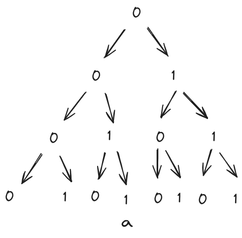
Binary codes are sequence of binary numbers $0, 1$ that encode human understandable information (characters, etc,) to electronic computers. Think of binary codes graphically as a path in a built binary tree, where leaves point to characters, and each paths to leaf is a binary code for that character.
For example, for the binary codes tree below, binary code for character $\mathbf{a}$ is $0011$. As a result, a list of characters can be represented by a sequence of their prefix-free binary codes. By prefix-free it means each character’s binary code is a path to leaf, no internal node in the tree, so there’s no conflict in prefixes of all binary codes.

In binary encoding, our objective is to use the shortest total or average length of binary numbers to encode a list of characters. Mathematically, for a list of characters $[s_1, s_2, …, s_n]$, denote their frequency probability as $[p_1, p_2, …, p_n]$, then our objective function is: \(\min_{s,\;p}\; B(S,P)=\frac{1}{n}\sum_i^np_i*len(s_i)\) where $len(s_i)$ denotes length of binary codes of $s_i$
this is actually a Greedy algorithm
The structured binary tree from this bottom up approach is the optimal binary codes that minimizes our objective $B(S, P)$.
Use Mathematical Induction method: assume number of characters in a set $n>=2$. When $n=2$, obviously Huffman Codes is correct.
When $n\geq3$, we need to prove Huffman Codes is correct when $n=k+1$ if Huffman Codes is correct when $n=k$, $\forall{k}\in{(3,4,…,n)}$. If Huffman Codes is correct when $n=k$, when $n=k+1$, merge the $s_1$, $s_2$ with the lowest two frequencies to $s_{12}$, now the character set is $S((12),3,4,…n)$ and $n=k$.
According to our assumption, when $n=k$, Huffman Codes tree $B(S_{12, 3,…,k}, P)$ is an optimal binary codes tree (that minimizes average binary code length). So we only need to prove: based on $B(S_{12, 3,…,k}, P)$ with $s_{12}$ is the merge of two lowest frequency character $s_1$, $s_2$, when $s_{12}$ is split into two child nodes $s_1$ and $s_2$, thus $n=k+1$, the binary codes tree is still optimal and it’s still Huffman Codes.
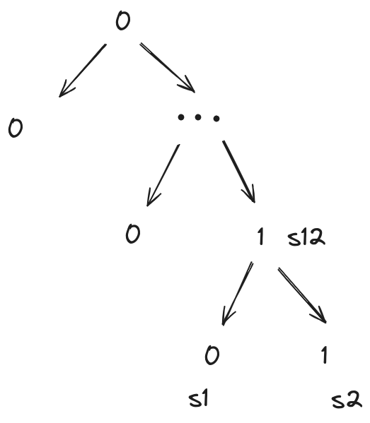
To prove $B(S_{1, 2, 3,…,k}, P)$ is Huffman Codes, since $B(S_{12, 3,…,k}, P)$ is optimal Huffman Codes, we only need to prove $s_1$, $s_2$ are at the deepest of the tree. Assume they are not, then there are $s_i$, $s_j$ that are deeper and have lower frequencies. This violates the assumption $s_1$, $s_2$ are the ones with lowest frequency. Thus $B(S_{1, 2, 3,…,k}, P)$ is Huffman Codes.
To prove $B(S_{1, 2, 3,…,k}, P)$ is optimal binary codes tree, assume there exists $B^{‘}(S_{1, 2, 3,…,k}, P)$ that makes $B^{‘}<B$, and $s_1^{‘}$, $s_2^{‘}$ are not the two with lowest frequencies $p_1^{‘}$, $p_2^{‘}$, because $B(S_{1, 2, 3,…,k}, P) = B(S_{12, 3,…,k}, P)+p_{1}+p_{2}\leq B(S_{12, 3,…,k}, P)+p_1^{‘}+p_{2}^{‘}=B^{‘}(S_{1, 2, 3,…,k}, P)$, there’s a better $B$ than $B^{‘}$. Therefore assumption fails. $B(S_{1, 2, 3,…,k}, P)$ is optimal binary codes tree.
class HuffmanTree:
	def __init__(self):
		self._root, self._codes = None, None
		self._maxDepth, self._minDepth, self._avgDepth = 0, 0, 0

	def encode(self, symbols=None):
		"""
		Huffman-encoding symbols
		symbols: [(w1, s1), (w2, s2), ..., (wn, sn)] where wi, si are ith symbol's weight/freq
		"""
		pq = MinHeap()
		symbols = copy.deepcopy(symbols)
		symbols = [(s[0], HuffmanNode(value=s[1], left=None, right=None)) for s in symbols]  # initialize symbols to nodes
		pq.heapify(symbols)
		while len(symbols) > 1:
			l, r = pq.pop(symbols), pq.pop(symbols)
			lw, ls, rw, rs = l[0], l[1], r[0], r[1]  # left weight, left symbol, right wreight, right symbol
			parent = HuffmanNode(value=None, left=ls, right=rs)
			pq.add(heap=symbols, item=(lw+rw, parent))
		self._root = pq.pop(symbols)[1]  # tree is complete, pop root node
		self._symbol2codes()  # create symbol: code dictionary
		self._maxDepth = len(max(self._codes.values(), key=len))  # max depth
		self._minDepth = len(min(self._codes.values(), key=len))  # min depth
		self._avgDepth = sum([len(d) for d in self._codes.values()]) / len(self._codes)  # mean depth

	def _symbol2codes(self):
		self._codes = dict()
		self._getCodes(self._root, '')

	def _getCodes(self, node, code):
		if not node.right and not node.left:
			self._codes[node.value] = code
			return
		self._getCodes(node.left, code+'0')
		self._getCodes(node.right, code+'1')

	@property
	def maxDepth(self):
		return self._maxDepth

	@property
	def minDepth(self):
		return self._minDepth

	@property
	def avgDepth(self):
		return self._avgDepth

	@property
	def root(self):
		return self._root

	@property
	def codes(self):
		return self._codes
for a set of numbers $a_1, a_2, …, a_n$ and its frequencies $f_1, f_2, …, f_n$, its constructed Optimal Binary Search Tree (sometimes called Weight-Balanced Binary Search Tree because it accounts for element weight/frequency/cost) is a binary search tree that maintains following property:
Optimal Binary Search Tree in principal is a sorted array. It is fast at element lookup in a set.
Consider a tree whose general structure like follow:
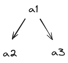
Let a series of set element be $a_1, a_2, …, a_n$, their frequencies be $f_1, f_2, …, f_n$, and 2 2-D arrays be $A$, $F$ where $A_{i, j}$, $F_{i, j}$ is the respectively the structure and minimum total frequencies for a Optimal Binary Tree consisting of elements $a_i, a_{i+1}, …, a_j$ ($i<=j$).
To divide the problem into sub-problems, notice for OBST $A_{i, j}$, it should be in a structure where root node is $a_k$, left child is $A_{i, k-1}$, and right child is $A_{k+1, j}$.
Why left child and right child are still optimal sub tress? For a optimal binary search tree $A_{i, j}$ with root $a_k$, if its right child node is not $A_{k+1, j}$, then there exists a better sub-tree, $A_{k+1, j}$, that makes total cost of $A_{i, j}$ less. Therefore the left child must be optimal sub tree. Same for right child.
Then for each tree $A_{i, j}$, and its cost $F_{i, j}$, we know ($F_{x, x-1}=0$)
\[F_{i,j}=\min_{\forall{k}\in{[i,...,j]}}\{F_{i,k-1}+F_{k+1,k}+\sum_{l=i}^{j}{f_l}\}\]When a $k$ is solved for each pair of $i, j$, the $k$ is the root value for the Optimal Binary Search Tree $A_{i, j}$. After we solve each root value for all $A_{i, j}$, we can break down any optimal binary search tree $A_{i, j}$’s structure from top to bottom.
now consider also unsuccessful search like following:
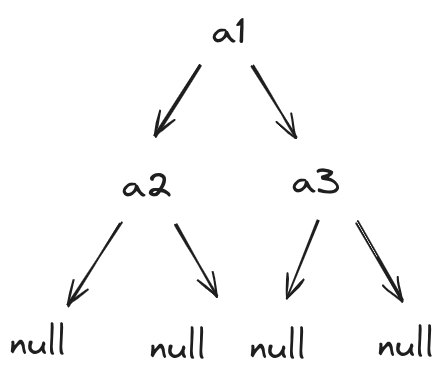
Null nodes are unsuccessful searches. For an OBST with N internal nodes (for successful searches), there are N+1 null nodes (for unsuccessful searches). The rules to divide the tree construction problem into subproblems that we noticed remain the same. That is:
for each tree $A_{i, j}$, and its cost $F_{i, j}$, we know ($F_{x, x-1}=0$)
\[F_{i,j}=\min_{\forall{k}\in{[i,...,j]}}\{F_{i,k-1}+F_{k+1,k}+\sum_{l=i}^{j}{f_l}+\sum_{m=i}^{j+1}{f'_m}\}\]where there’s an additional sum term for $f’_m$, $m\in{[i, j+1]}$ which is sum of frequency for all Null Nodes.
we can use dynamic programming to construct an Optimal Binary Search tree for ${a_1, a_2, …, a_n}$ and calculate its cost. The pseudo code is:
for {d=0; d<=n; d++}{
	for {i=0; i<=n-d; i++}{
		// F[i][j] is total cost for OBST consisting elements {ai,..,aj}. F[X][X-1]=0.
		// Could use extra space to denote F[x][x] as 0 (no element) and F[x][x+1] as total frequency of elements {x}
		// W[i][j] is total frequency for elements  {ai,...,aj}. It includes Null Nodes if uncessful searches are considered and corresponding frequencies are given.
		F[i][i+d] = min{F[i][k-1] + F[k+1][i+d]} + W[i][j] for any k in {i, ..., i+d}
		A[i][i+d] = optimal k // root element number for this tree cosisted of elments {i, i+1, ..., i+d}
	}
}
First of all, B tree is a M-way tree, it can have more than 2 child nodes for each node. The similarity is that during an element search down the tree, node value is being compared to determine where to go down the path. B/B+ tree is commonly used in multi-level indexing database system where a search/query can quickly locate the searched element’s address in hard disk. OBST can be used where one needs a data structure that supports fast array element lookup.
First, the objectivity is totally different: OBST is for quick set element lookup whereas Huffman Codes are for efficient data encoding such as file compression. In other words, Huffman Codes encode a series of characters/elements, or an array, into binary codes where total numbers of binary digits needed are at optimal/minimum. Huffman Codes is not for quick array element search which is OBST’s purpose.
Union-find, or disjoint-set, is a tree structure that supports fast categorization/grouping (the ‘union’) and group id lookup for a member (the ‘find’). It is a tree because it uses path compression to balance a tree structure to efficiently iddentity group an element belongs to.
S1 = Find(x)
S2 = Find(y)
if rank(S1) > rank(S2){
parent[S2] = S1
} elif rank(S1) < rank(S2){
parent[S1] = S2
} else {
parent[S2] = S1
ranks[S1] += 1
}
class Union:
    def __init__(self, n):
        self.p = [i for i in range(n)] # parent
        self.r = [0 for i in range(n)] # rank for path balancing

    def find(self, i):
        if self.p[i] != i:
            return self.find(self.p[i])
        return i

    def union(self, i, j):
        ri, rj = self.find(i), self.find(j)
        if ri == rj:
            return
        r = self.r
        p = self.p
        if r[ri] < r[rj]:
            p[ri] = rj
        elif r[rj] < r[ri]:
            p[rj] = ri
        else:
            p[rj] = ri
            r[ri] += 1
Hash Tables are a data structure of constant size whose indexes are within a fixed range and are hash values from hash functions with element as input. The more evenly distributed the hash values are, the more efficient the hash table can be.
Load Load of hash table = # of objects in hash table / # of slots of hash table
Advantages: $O(1)$ in insertion, deletion, lookup
Setup Universe set U, an arbitrary size of input (key)
Goal Maintain evolving set S « U (a fixed size of hash values from key through hash function)
Solving collision by
i++ and rehash until no collision; in search, search element from $i=0$, if not found, i++ and rehash until element found (or all $i$ is traversed?). Time Complexity of Insertion and Search in this probing will be O(K) where k is maximum i.A variant of Hashing to extremely fast check whether an element is a member of a set with a certain (high) accuracy. For examples, check availability of username during account registration.
Given data set S:
| array of bits | 0 | 0 | 0 | 0 | 0 | 0 | 0 | 0 | 0 | 0 |
|---|---|---|---|---|---|---|---|---|---|---|
| hash | 1 | 2 | 3 | 4 | 5 | 6 | 7 | 8 | 9 | 10 |
Assumption All hash function $h_{i}\left( x \right),\ i\ = 1,\ 2,\ \ldots,\ K$ generate random keys uniformly distributed across the table.
Analysis
Denote Set A as the bloom filter array, $A_{1},\ A_{2},\ A_{3},\ \ldots,\ A_{n}, = \ \ 0\ or\ 1$
Denote Storage space is array A of n bits, one bit per hash value
Denote Input data set S that’s inserted, length = S
\(P\left( A_{i} = \ 1 \right) = 1 - \left( 1 - \frac{1}{n} \right)^{K\left| S \right|},\ \forall\ i \in 1,\ 2,\ 3,\ \ldots,\ n\)
Because $e^{- \frac{1}{n}} > 1 - \ \frac{1}{n}$
\(P\left( A_{i} = \ 1 \right) \leq 1 - e^{- \frac{1}{n}K\left| S \right|},\ \forall\ i \in 1,\ 2,\ 3,\ \ldots,\ n\)
Let b be number of bits allocated to each object in input set S: $b = \ \frac{n}{S}$ > 0
Therefore,
\(P\left( A_{i} = \ 1 \right) \leq 1 - e^{- \frac{K}{b}},\ \forall\ i \in 1,\ 2,\ 3,\ \ldots,\ n\)
So $for\ x \notin S$
\(p\left( \text{false\ positive\ of\ x} \right) = \ \coprod_{i = 1}^{K}{P\left( h_{i}\left( x \right) = 1 \right)} \leq \ \left\lbrack 1 - \ e^{- \frac{K}{b}} \right\rbrack^{K},\ \forall\ x \notin S\)
Objective
\(\min{p\left( \text{false\ positive\ of\ x} \right)},\ \forall\ x \notin S\)
\(\min\left\lbrack 1 - \ e^{- \frac{K}{b}} \right\rbrack^{K},\ \forall\ x \notin S,\ K \geq 1,b \geq 1\)
Set b constant, (what’s usually determined or if not, to find relationship between K and b), and define:
\(f\left( x \right) = \left\lbrack 1 - \ e^{- \frac{x}{b}} \right\rbrack^{x},x \geq 1,b \geq 1\)
First derivative:
\(f^{'}\left( x \right) = e^{ln(1 - e^{- \ \frac{x}{b}})x}\lbrack\frac{e^{- \ \frac{x}{b}}*\frac{1}{b}*x}{1 - e^{- \frac{x}{b}}} + ln(1 - e^{- \ \frac{x}{b}})\rbrack\)
x>=1, b>=1
Note the left part of the left formula
\(e^{ln(1 - e^{- \ \frac{x}{b}})x} > 0\)
We only need right part of the left formula to know f(x) monotony.
Define:
\(g\left( x \right) = \frac{e^{- \ \frac{x}{b}}*\frac{1}{b}*x}{1 - e^{- \frac{x}{b}}} + \ln\left( 1 - e^{- \ \frac{x}{b}} \right),\ x > = 1,\ b > = 1\)
Let: \(y = 1 - \ e^{- \ \frac{x}{b}},x \geq 1,b \geq 1\)
In order to know f(x) monotony, we only need to know g(y) range.
Namely to know range of:
\(h\left( y \right) = \left( 1 - y \right)^{\frac{y - 1}{y}}*y - 1,y \in (0,1)\)
To know range of h(y), let’s try looking at its monotony by its first
derivative:
\(h^{'}\left( y \right) = \frac{1}{y}*e^{\ln\left( 1 - y \right)*\frac{y - 1}{y}}*\left\lbrack 2y\ + \ln\left( 1 - y \right) \right\rbrack,\ y \in (0,1)\)
Note left part of the right side of equation:
\(\frac{1}{y}*e^{\ln\left( 1 - y \right)*\frac{y - 1}{y}} > 0\)
Define:
\(k\left( y \right) = 2y\ + \ln\left( 1 - y \right),\ y\ \in (0,\ 1)\)
Then its first derivative:
\(k^{'}\left( y \right) = - \frac{1}{1 - y} + 2,\ y \in (0,1)\)
Easily know:
\(k^{'}\left( \frac{1}{2} \right) = 0\)
\(k^{'}\left( y < \frac{1}{2} \right) > 0\)
\(k^{'}\left( y > \ \frac{1}{2} \right) < 0\)
Therefor:
k(y) monotically increase at (0, 0.5) and monotically decrease at (0.5, 1)Note that there’s a number between 0.5 and 1 that make the function equal to zero,\
Denote it as a constant a, so:
\(1 > \ a > 0.5\)
\(k\left( a \right) = 0\)
By extreme value we know:
\(k\left( y \right) > 0,\ y \rightarrow 0\)
Therefore,
\(k\left( y \right) > 0,\ y \in (0,\ a)\)
\(k\left( y \right) < 0,y \in (a,1)\)
Namely,
\(h'\left( y \right) > 0,\ y \in (0,\ a)\)
\(h'\left( y \right) < 0,y \in (a,1)\)
Namely
h(y) monotically increase at (0, a) and monotically decrease at (a, 1)
a is a constant and 1 > a > 0.5Obviously:
\(h\left( 0.5 \right) = 0\)
So,
\(h\left( y \right) < 0,\forall\ y \in (0,\ 0.5)\)
Consider when 1 > y > 0.5,
\(h\left( y \right) = \ \left( 1 - y \right)^{\frac{y - 1}{y}}*y - 1,y \rightarrow 1\)
\(h\left( y \right) = \ \left( 1 - y \right)^{\frac{y - 1}{y}} - 1,y \rightarrow 1\)
\(h\left( y \right) \rightarrow 0\)
Therefore,
\(h\left( y \right) > 0,\ \forall\ y \in \ \left( 0.5,\ 1 \right),\ *not\ a\ very\ strict\ proof\)
To sum up,
\(h\left( y \right) < 0\ \forall\ y \in \left( 0,\ 0.5 \right),\ h\left( y \right) = 0\ for\ y = 0.5,\ h\left( y \right) > 0\ \forall\ y \in (0.5,\ 1)\)
Obviously,
\(g\left( y \right) < 0\ \forall\ y \in \left( 0,\ 0.5 \right),\ g\left( y \right) = 0\ for\ y = 0.5,\ g\left( y \right) > 0\ \forall\ y \in \left( 0.5,\ 1 \right)\)
Namely,
\(f'\left( y \right) < 0\ \forall\ y \in \left( 0,\ 0.5 \right),\ f'\left( y \right) = 0\ for\ y = 0.5,\ f'\left( y \right) > 0\ \forall\ y \in (0.5,\ 1)\)
Namely:
f(y) monotically decrease at (0, 0.5) and monotically increase at (0.5, 1)
Therefore,
\(\min{f\left( y \right)} = f\left( 0.5 \right)\)
Therefore,
\(1 - \ e^{- \ \frac{x}{b}} = 0.5\)
So
In all, when number of hash functions $K = ln2 * b$ ($b$ is number of bits allocated per object key), ($ln2 = ~0.693$). Then, Bloom Filter’s FPR for new insert $x$ is at its minimum (assume S is inserted already).